---

GIS Analyses

The GIS analyses can be broken into two parts: the data preparation, which included projecting, georeferencing and digitizing, and the analysis, which included the least-cost analysis. We present general steps of how the analyses were done, so that hopefully you can repeat the same analyses on these data or your own data from another location.

Data Preparation

Analysis

---

Data Preparation:

1) Ethiopian DEM

2) Topo Map

3) Georeferencing the TIFF image

4) Digitizing

5) Clipping a DEM to the size of Murile_Topo

6) Converting Vector Data to Raster Data

Ethiopian DEM:

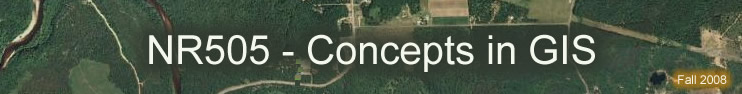
We obtained an un-projected 90 m Digital Elevation Model (DEM) of Ethiopia from the class network drive and re-projected it to UTM Zone 37 N, WGS84:

Open ArcCatalog, use the Define Projection tool found in the ArcToolbox.

Topo Map:

We met with members of the Murulle Foundation and the Ethiopian Rift Valley Safaris who marked locations of water access and village locations on a paper topographic map of the Murile Region.  This map was then scanned and saved to disk as a PDF document. 

Using Adobe Acrobat Professional the PDF was exported as a TIFF file.

Georeferencing the TIFF image:

Open ArcMap and add the re-projected DEM to a blank map (this sets the data frame's coordinate system to that of the DEM: UTM Zone 37 N, WGS84). Add the scanned topo map TIFF to the map. Activate the georeferencing toolbar.

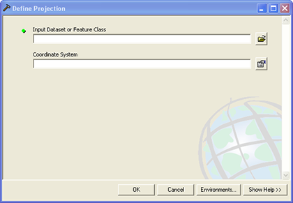
Select the control point tool to link two points of known degrees, minutes, seconds (DMS) coordinates on the scanned topo map TIFF to the UTM Zone 37 N coordinates of the data frame. 

Use a DMS to UTM conversion tool, such as: DMAP Transverse Mercator Calculator to calculate the destination coordinates of the control points. Enter these destination coordinates via key input rather than a mouse click (right click and select: 'input x and y…'). 

Select 'Update Georeferencing' from the 'Georeferencing' pull-down menu.  Now the map is georeferenced. As a check see if the topography from the scanned map lines up well with the topography generated from the DEM. 

Save the georeferenced map as a layer file (Right click on the georeferenced map in the table of contents and save as layer file…).  We named it Murile_Topo.

Digitizing:

Before digitizing can take place we need to create new Feature Classes to hold our digitized data:

Point locations including the water access points and village locations were digitized as point vector data: 

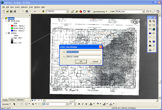
In ArcCatalog create a geodatabase to hold all the data for the project, we called our database CostAnalysis_Murile.mdb.  Create a new Feature Dataset (right click on the geodatabase, select: 'New', 'Feature Dataset…').

Name it something logical for example: WaterSourcePts. 

Within this new Feature Dataset create a new Feature Class (right click on the Feature Dataset, select: 'New', 'Feature Class…').  Name the feature class appropriately such as: Water1 and select ‘point features’ from the ‘Type’ pull-down menu.  Accept the defaults. Continue to create new point features for all the water resource points and the village locations, placing them in appropriate feature datasets and labeling them in a logical way.

The Omo River is a polyline feature so it was digitized as line vector data:

In ArcCatalog open your geodatabase and create a new Feature Dataset (right click on the geodatabase, select: 'New', 'Feature Dataset…').  Name it something logical for example: Streams_Water.  Within this new Feature Dataset create a new Feature Class (right click on the Feature Dataset, select: 'New', 'Feature Class…').  Name the feature class appropriately: OmoRiver and select ‘polyline features’ from the ‘Type’ pull-down menu.  Accept the defaults. 

Dipa Lake is a polygon feature so it was digitized as polygon vector data: 

In ArcCatalog open your geodatabase and expand to the Streams_Water Feature Dataset.  Within this Feature Dataset create a new Feature Class (right click on the Feature Dataset, select: 'New', 'Feature Class…').  Name the feature class appropriately: DipaLake and select ‘polygon features’ from the ‘Type’ pull-down menu.  Accept the defaults. 

Close AcrCatalog and open ArcMap, add the new Feature Classes (i.e. Water1) to a new map that includes the georeferenced topomap (Murile_Topo).  Enable the Editor toolbar:

Each of these new Feature Classes are now empty (do not contain any data) and are ready to hold digitized data:

In the editor toolbar select 'start editing' from the 'Editor' pull-down menu. Select 'create new feature' in the 'Task' pull-down menu and select one of the new empty Feature Classes (such as Water1) from the 'Target' pull-down menu. Next select the sketch tool from the Editor Toolbar.

For the point features: Left click with the mouse on each point of the Murile_Topo map that you wish to include in your current target feature class. For example, with Water1 click on the most northern water access point, and you're done!

For the polyline features: Left click with the mouse at the starting point of the line feature on the Murile_Topo map that you wish to include in your current target feature class. Continue to click along the line feature until the end is reached. Double click at the last point to end the line. Example: OmoRiver.

For the polygon features: Left click with the mouse somewhere on the edge of the polygon feature on the Murile_Topo map that you wish to include in your current feature class. Continue to click around the perimeter of the polygon until you get back to the original starting point. Double click near the original point to close the polygon. Example: DipaLake.

When you are done digitizing the contents of each of these feature classes, select 'Save Edits' from the 'Editor' pull-down menu on the Editor Toolbar.

Clipping a DEM to the size of Murile_Topo:

The 90 m DEM we obtained covers the entire South Omo region of Ethiopia. We only need the DEM data for the area that the Murile_Tope map covers, this will conserve computing power during the rest of our analysis and save time.

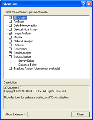
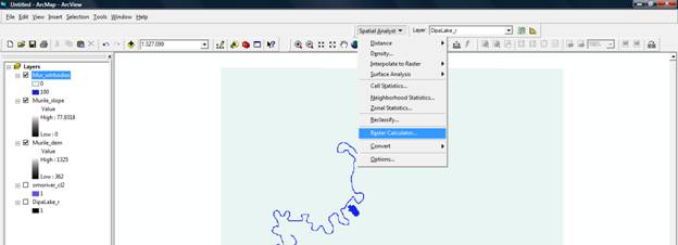
Open ArcMap and add Murile_Topo and the 90 m DEM data to a blank map. Select 'Extensions' from the Tools menu and activate the Spatial Analyst extension. Activate the Spatial Analyst toolbar.

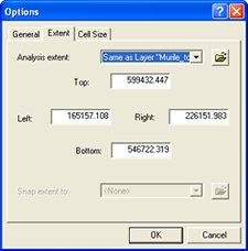
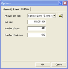
Select 'Options' from the pull-down 'Spatial Analyst menu. In the 'General' tab set an appropriate working directory for your data to be saved in (the geodatabase is a great idea). On the 'Extent' tab select the Murile_Topo from the 'Analysis Extent:' pull-down box. On the 'Cell Size' tab select the DEM from the the 'Analysis Cell Size:' pull-down box. Click OK.

Select 'Raster Calculator' from the 'Spatial Analyst' menu.

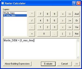
Type: 'name of DEM clip = [DEM]' (for example, we named ours: 'Murile_DEM = [S_omo_dem]') and click 'Evaluate'. This will create a new DEM raster with the spatial extent of the Murile_Topo and with the same cell size as the original DEM.

Converting Vector Data to Raster Data:

The data we have created through digitizing is in vector format. We need to convert these data to raster format in order to perform our cost-distance analyses:

Open Arcmap and add the vector data you have just created to a new blank map. Activate the ArcToolbox and expand 'Conversion Tools', 'To Raster'. The point features require the 'Point to Raster' tool.

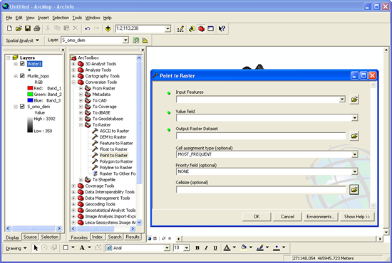
Select the Point Feature Class you wish to convert to a raster from the 'Input Features' pull-down box. change the output file name to something appropriate in the 'Output Raster Dataset' box. Accept all other defaults, except the cell size.

The cell size should be the same as the cell size for the DEM being used in the analysis. You can copy the exact cell size by going back into the 'Cell Size' tab of the 'Spatial Analyst' pull-down menu 'Options'. Enter this cell size into the cell size box. Click OK.

Perform a similar operation to convert the Polyline and Polygon vector data to raster data. The tools for these Feature Classes can be found in the same part of the ArcToolbox. Again, be sure to set the cell size to the cell size of the DEM being used in the analysis and save your files with appropriate names.

We are now ready to begin our Least-Cost Analysis.

Return to top

Data Preparation

Analysis

---

Analysis:

1) Reclassify & mosaic raster data

2) Create slope raster

3) Combine slope & water bodies rasters

4) Least-cost analysis

Reclassify & mosaic raster data:

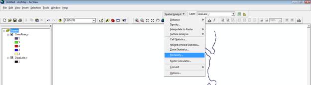
Open ArcMap and add data: OmoRiver_r & DipaLake_r using the ‘Add Data’ button: 

Make sure that the Spatial Analyst Extension is turned on.

Then, open the Spatial Analyst toolbar.

Reclassify data in OmoRiver_r raster data set so that all values are 1s (river) and 0s (no river).

First choose ‘Reclassify’ under the ‘Spatial Analyst’ toolbar.

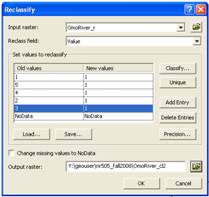
Within the ‘Reclassify’ window, choose the OmoRiver_r raster as the Input Raster, and make sure the ‘Reclass field’ is set to ‘Value.’ Then, manually change the New values to ‘1’ for all Old values with data. Then choose an appropriate name to save the raster and click OK.

Now, we will mosaic the reclassified OmoRiver_r raster with the DipaLake_r raster, so that there is one raster with all the water bodies with a value of ‘1.’

Open the Raster Calculator in the Spatial Analyst toolbox.

Within Raster Calculator, write an expression to mosaic the DipaLake_r and reclassified OmoRiver_r rasters into a new raster and give it an appropriate name (eg. Mur_ wtr_uncl2, which means Murile water- unclassified). Click on ‘Evaluate.’

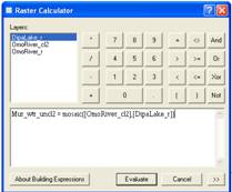
*Tip: You can insert the raster files to be combined by double-clicking on the raster files in the list (top-left). Also, make sure there is a space on both sides of the equal (=) sign.

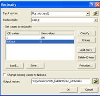
We will use this raster to add to the slope raster to be used in the least-cost analysis, so that least cost paths avoid the water bodies. In order for the least cost analysis to know that the water bodies should be avoided, we want this to have a very high percent slope value. Therefore, we will reclassify this raster so that the ‘1’ values are now set to ‘100,’ and the rest of the values, including ‘no data,’ have a value of ‘0.’

Create slope raster :

Next, add the Murile region DEM (Murile_DEM)

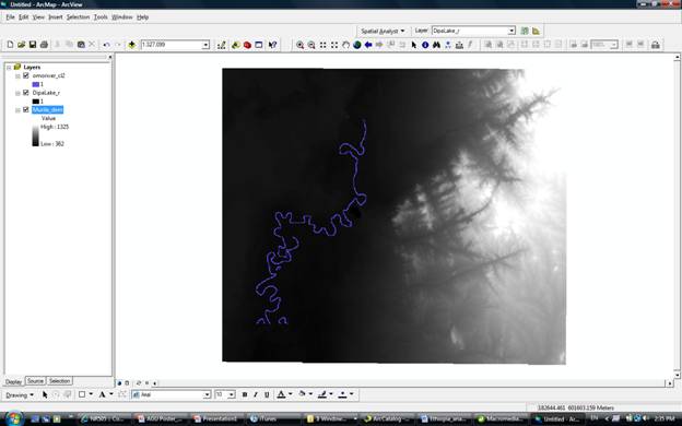
We will now use 'Spatial Analyst' to convert this DEM into a slope raster, showing the slope of the hillside in percent.

Under the ‘Spatial Analyst’ choose ‘Surface Analysis’ and then ‘Slope…’

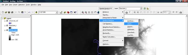
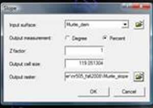
Choose the ‘Input surface’ as the DEM being used (Murile_dem), and whether you would like the values in degrees of percent. Finally, choose a meaningful name for the ‘Output raster.’

Combine slope & water bodies rasters:

In order for the cost-direction grid to avoid water bodies, we will create a new slope raster (wtrslope) where the slope raster is added to the reclassified .

Add the rasters: Mur_wtrbodies & Murile_slope and open the ‘Raster Calculator.’

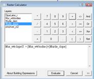
Write a statement to add the Mur_wtrbodies raster to the Murile_slope raster. Give it a meaningful name. This raster name has a ‘U’ for ‘unclassified.’ In the next step we will reclassify this raster.

*Tip: Make sure there are spaces on both sides of the '=' and '+' signs.

In order to make all of the waterbodies equally costly, we want to reclassify this raster so that all values above 100, will be set to 100. Instead of using the 'reclassify' option, we will write a 'con' statement within the 'Raster Calculator.'

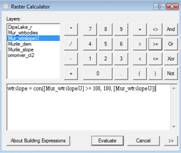
Write a ‘con’ statement to reclassify the ‘Mur_wtrslopeU’ raster. This statement creates a new raster, where all values greater than or equal to 100 are classified as 100.

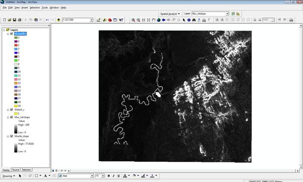
Keep the Mur_wtrslope and Murile_slope rasters. Add the Water1_r and Vill_les20_r rasters. Because the village raster is classified into 19 different values, we will need to reclassify this raster so they all have a value of 1. Use the ‘Reclassify’ option to do this. See steps above to see how to do this.

Least-cost analysis:

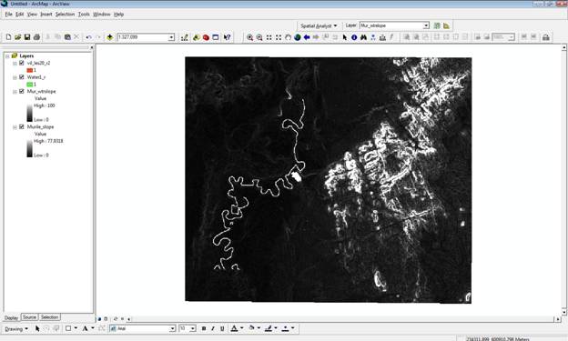
To be ready for the least-cost analysis, your map document should look like the one below and the following three rasters will be used: reclassified villages raster (vil_les20_r2), water source 1 (Water1_r), and Mur_wtrslope.  Any other files may be open if it helps to visualize the analysis.

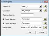
First, we will created a cost-weighted distance grid for our 'source' point, the 'Water1_r' raster.

In the 'Cost Weighted' box, choose the water source (Water1_r) as the 'Distance to:' and the Mur_wtrslope as the 'Cost raster.' The direction and allocation rasters can be temporary and give the output raster a meaningful name.

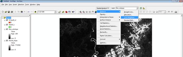
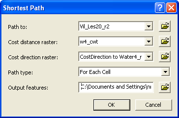
After the cost direction and cost allocation grids are created, it is time to create the shortest path. Under the 'Spatial Analyst' toolbar, choose 'Distance' and 'Shortest Path.' Enter the villages raster (Vil_les20_r2) as the 'Path to:', the 'Cost distance raster' is the raster created as the direction raster in the previous step. The 'Cost direction raster' is the temporary 'direction' raster created. Choose 'For each Cell' as the 'Path type,' and finally choose a meaningful name to save your final path.

The final path created will then show up as a line vector file.

Return to top

Data Preparation

Analysis