GIS Concepts and Examples of Their Use in This Analysis |
The following explanations of concepts are excerpted from ArcGIS 9.2 ArcCatalog Desktop Help
GIS Anaylses
We used both raster and vector analyses in this demonstration project.
Raster files are made up of pixels and have an associated resolution that is usually expressed as the number of pixels per inch (dpi). Raster files are best at containing images that are made up of many different colors such as photographs or satellite images. They do not scale well and can appear blocky or jaggy if increased in size. Raster file exporters included with ArcMap are BMP, TIFF, JPEG, GIF, and PNG.
Vector files are made up of mathematical descriptions of objects such as points, polygons, lines, and text. Vector files scale well since they do not have an associated resolution and they will look the same at whatever size they are displayed. Vector files can also contain raster images, although the raster portions may not scale as well as the vector portions. Vector file exporters included with ArcMap are EMF, EPS, PDF, AI, and SVG. Vector files are generally smaller in size than a corresponding raster file.
View Data Schematic and Naming Conventions
GIS Concepts in the Literature
Much of our conceptual knowledge about GIS concepts in this class comes from Longley et al.’s book Geographic Information Systems and Science and Theobald’s GIS textbook, GIS Concepts and ArcGIS Methods. An example of the value of GIS in everyday management and conservation in the National Park Service is Henry and Armstrong’s text Mapping the Future of America’s National Parks. Many of the projects in the book illustrate applications related to natural resource management throughout the Service and provide a basis for demonstration projects such as this.
General GIS Analysis
This analysis applies to both vector and raster data.
Project
Project changes the coordinate system of your Input Dataset or Feature Class to a new Output Dataset or Feature Class with the newly defined coordinate system, including the datum and spheroid. Any datasets or feature classes used in analysis must be in the same projection.
For this analysis, we used North American Datum 1983 (geographic coordinate system). The state of Hawaii crosses two universal transverse mercator (UTM) zones – 4N (Haleakala National Park, Kalaupapa National Historic Park) and 5N (Hawaii Volcanoes National Park). Therefore, we occasionally had to reproject the same feature class in both 4N and 5N (the ocean, for example), so that it could be used in display and analysis for the respective parks.
Vector Analyses
Buffer
Buffer is a proximity analysis that creates “buffered” polygons to a specified distance around the Input Features, which can be polygons, lines, or points. An optional “dissolve” can be performed to remove overlapping buffers.
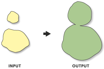
An example of buffering in this project includes buffering the lava polygon in Hawaii Volcanoes National Park by ½ mile. This buffer represented an area that is likely not “safe” for any future Ischaemum byrone restoration efforts. |
Clip
Clip is used to cut out a piece of one feature class using one or more of the features in another feature class as a "cookie cutter". This is particularly useful for creating a new feature class that contains a geographic subset of the features in another, larger feature class.
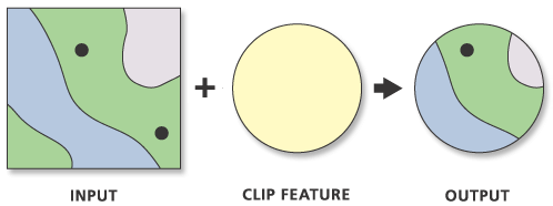
Examples of clipping in this project include clipping roads, trails, rivers, and lava to a park’s boundary. |
Dissolve
Dissolve analysis aggregates features based on specified attributes. Features with the same value combinations for the specified fields will be aggregated (dissolved) into a single feature.
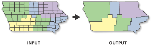
An example of when dissolve was used in this analysis is when the area of all a park’s buffered ‘threats’ (lava, structures, roads, threats, etc.) were combined, or unioned, and then aggregated, or dissolved, to get a total area that represented all threats.
|
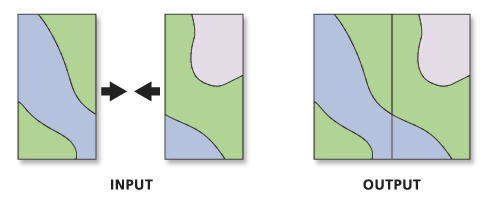
Union
Union analysis computes a geometric intersection of the Input Features. All features will be written to the Output Feature Class with the attributes from the Input Features, which it overlaps.
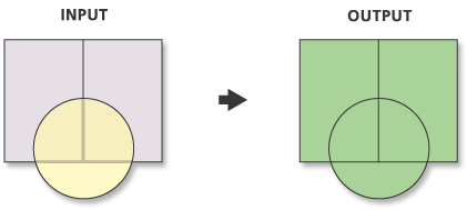
An example of a union in this analysis is the combined threat coverage for all three parks, where all perceived threats to Ischaemum byrone populations in each park were buffered and then combined, or unioned, to get one layer that represented multiple threats.
|
Merge
Merge combines input features from multiple input sources (of the same data type) into a single, new, output feature class. The input data sources may be point, line, or polygon feature classes or tables.
Merge was used in this analysis to combine two Ischaemum byrone population point features into one feature that shows extant populations in Hawaii Volcanoes National Park.
|
Spatial Query
Select by Attribute: There are various ways to select features in ArcMap. One way is to select features through an attribute table. From a table, you can interactively select records by pointing at them, or you can select those records that meet some criteria, for example, find all soil types that are pahoehoe or a’a lava.
Once you've defined a selection, you'll see those features highlighted on your map. For example, we wanted to find the most recent age of lava for a particular volcano in Haleakala. First, we sorted the geologic records in the table to find Haleakala volcano. Then we sorted that selection by rock type (lava). We then performed another ‘select within selection’ for all rock types with an age class of ‘1’, which was the youngest lava rock. We then created a shapefile form this final selection and added it to the dataset.
Select by Location: lets you select features based on their location relative to other features. For example, we selected the relevant islands (the Big Island, Maui, and Molokai) from all islands of the State of Hawaii.
|
Raster Analyses
Spatial Analyst
This ArcGIS extension provides a comprehensive set of advanced spatial modeling and analysis tools that allow you to perform integrated raster and vector analysis. The following tools were used in this project:
- Hillshade: A type of surface analysis that allows the user to examine the raster’s shaded relief. We performed hillshade analysis for all three parks to use in the map displays (e.g. KALA_hlshd).
- Raster calculator: The raster calculator enables you to perform many different types of queries on your data. For example, we used a conditional statement to return grid cells that fit our stated criteria (0-250 elevation). An example of one of the raster calculator equations we used is “HAVO250a=con([project_HAVO]<=76.22,[project_HAVO])” which identified all those cells of the elevation raster that are lower than 76.22 meters (equals 250 feet). Those cells that met the criteria were given a value of 1 in the output raster. Cells that do not meet the criteria (cells with elevations higher than 76.22 meters) were given a value of 0 in the output raster.
- Reclassify: Reclassifying data changes cell values by replacing input cell values with new output cell values. We reclassified the raster grids for all three parks from their original elevation data and grouped certain values together, i.e. the elevation range we were interested in – 0-250 feet above sea level (e.g. grid name = KALA250).
|
Raster to Polygon
Converts a raster integer dataset to a polygon (vector) dataset. In this project, once we derived a raster that contained elevation data only between 0-250 feet ASL, we wanted to convert this to a polygon that could be incorporated into an area analysis that when intersected with soils data (when available) allowed the calculation of total area of suitable habitat for Ischaemum byrone in each park.
|
BACK TO HOME PAGE