DATA ANALYSIS

PAGE OUTLINE:

Critical Components
Initial Set-up
Data Analysis
Data Aquisition
Data Preparation

----------------------------------------------------------------------------------------------------------------------------

THREE CRITICAL COMPONENTS:

1. Amount of vegetation
The amount of vegetation coverage within each wolf pack can be directly related to the likelihood that a herdsman will take his cattle to graze on the land within that wolf pack. Thus, higher vegetation densities are associated with higher chances of cattle herding, and higher chances of cattle herding are associated with an increased risk (among the endangered wolves) of domestic dog contact. Increased domestic dog contact will significantly raise the chances of the wolves’ exposure to rabies, and this increase in exposure makes vegetation coverage an indirect rabies risk factor. To help assess the risk of rabies within each wolf pack, the amount of grazing vegetation (herbaceous coverage and grasslands) needs to be quantified. See the following steps for this part of our analysis.

2. Proximity to water
Water is a very important life resource. Just as areas of higher vegetation densities rank above those of lower densities (in terms of herding cattle), regions that have more abundant water resources will take priority over regions with fewer water resources. Our water proximity analysis is based on an 800-meter buffer placed around all streams within our wolf territory boundary. The area (in square meters) of stream buffer coverage within each wolf-pack’s polygon will be used to assess the desirability of each wolf-pack location for cattle herding.

3. Proximity to villages
Distance from surrounding villages is also a factor that needs to be integrated in our risk analysis. Herdsmen will most likely choose herding locations that are closest to their villages in order to reduce travel time and traveling distance. Since rabies risk decreases with increasing distance, we have chosen to use the inverse distance in our rabies risk equation.

----------------------------------------------------------------------------------------------------------------------------

INITIAL SET-UP:

Tools – Extensions – Turn on Spatial Analyst
Tools – Customize – Under the Toolbars tab, select Spatial Analyst

----------------------------------------------------------------------------------------------------------------------------

DATA ANALYSIS:

Amount of Vegetation

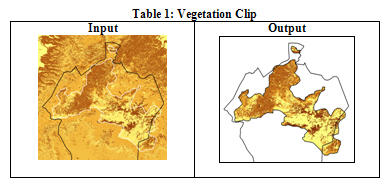
1. Clip vegetation map to wolf territories:

Set the following options (located in the Spatial Analyst drop-down menu, Options):

Working directory: Raster files folder

Analysis mask: Wolf_territories

Analysis extent: Same as Layer “Wolf_territories”

Analysis cell size: Same as Layer “Vegmap”

Open the Spatial Analyst Raster Calculator

Use the following expression to cut the vegetation raster to the wolf territory layer: VegMap_Clip = [Vegmap]

Join the Vegmap attributes to the VegMap_Clip attribute table so that vegetation types can be identified within the clipped vegetation raster.

Right-click the VegMap_Clip layer

Select Joins & Relates, and Join

Choose the layer to be joined and the common field in both layers to be joined

The VegMap_Clip displays types of vegetation within the wolf-pack territory boundaries.

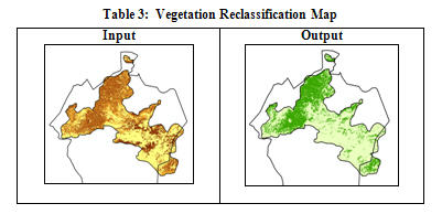
2. Create a Herbaceous and Grassland Vegetation Raster:

Use the Reclassify tool in the Spatial Analyst drop-down menu to change herbaceous and grassland categories to “1” and all others to “0”

Open the Raster Calculator and enter the following expression to create a herbaceous/grassland only raster: Veg_HerbGrass = SELECT ([Veg_Reclass], 'VALUE = 1')

Proximity to Water

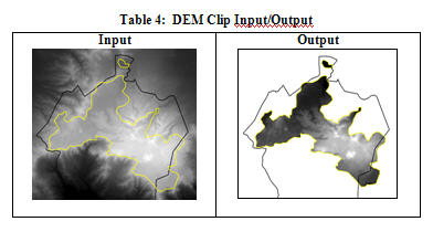
1. Clip DEM to wolf territories:

Set the following options (located in the Spatial Analyst drop-down menu, Options):

Working directory: Raster files folder

Analysis mask: Wolf_territories

Analysis extent: Same as Layer “Wolf_territories”

Analysis cell size: Same as Layer “dem”

Open the Spatial Analyst Raster Calculator

Use the following expression to cut the DEM raster to the wolf territory layer: DEM_Clip = [dem]

The DEM_Clip displays elevation within our wolf-pack territories. This area is characterized by elevations between 3,013 meters and 4,385 meters.

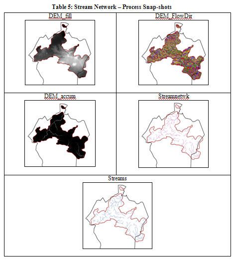
2. Create a stream layer for DEM:

Set Spatial Analyst settings (Spatial Analyst menu - Options)

Select the desired working directory

Analysis Mask: DEM_Clip

Analysis Extent: same as layer “DEM_Clip”

Analysis Cell Size: same as layer “DEM_Clip”

Complete the following sequence of steps:

Open ArcToolbox, expand Spatial Analyst Tools, Hydrology

Select Fill

Input surface raster: DEM_Clip

Output surface raster: DEM_fill

Select Flow Direction

Input surface raster: DEM_fill

Output surface raster: DEM_FlowDir

Select Flow Accumulation

Input raster: DEM_FlowDir

Output raster: DEM_accum

Create a stream network as a linear feature:

Enter the following expression in the Spatial Analyst Raster Calculator: Streamnetwk = con ([DEM_accum] > 100, 1)

Select Stream to Feature (Hydrology, under Spatial Analyst Tools, in ArcToolbox).

Input stream raster: Streamnetwk

Input flow direction raster: DEM_FlowDir

Output polyline features: Streams

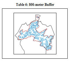
3. Create an 800-meter buffer that will represent the most desirable herding areas due to proximity to water:

Open ArcToolbox, expand Analysis Tools, Proximity, open Buffer

Input feature: Streams

Output feature: Stream_Buffer

Linear unit: 800 meters

Side type: Full

End type: Round

Dissolve type: All

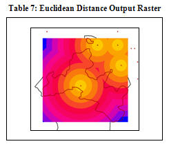
Proximity to villages

1. Create a continuous prediction surface based distance between Ethiopian towns:

Set Spatial Analyst settings (Spatial Analyst menu - Options)

Select the desired working directory

Analysis Mask: <none>

Analysis Extent: same as layer “Wolf_territory”

Analysis Cell Size: same as layer “Veg_HerbGrass”

Open ArcToolbox, expand Spatial Analyst Tools, Distance, select Euclidean Distance

Input feature source: Ethiopia_Towns

Output distance raster: Town_EucDist

Pulling it all Together

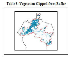
1. Clip Veg_HerbGrass layer using Stream_Buffer to create areas of highest priority for cattle herdsmen:

Set Spatial Analyst settings (Spatial Analyst menu - Options)

Select the desired working directory

Analysis Mask: Stream_Buffer

Analysis Extent: same as layer “Veg_HerbGrass”

Analysis Cell Size: same as layer “Veg_HerbGrass”

Enter the following expression in the Raster Calculator: Veg_Stm_Area = ([Veg_HerbGrass])

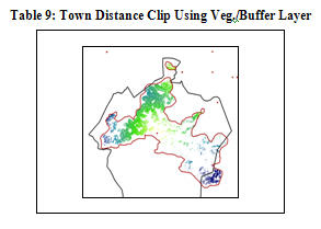
2. Clip the Town_EucDist layer using the Veg_Stm_Area layer:

Set Spatial Analyst settings (Spatial Analyst menu - Options)

Select the desired working directory

Analysis Mask: Veg_Stm_Area

Analysis Extent: same as layer “Veg_Stm_Area”

Analysis Cell Size: same as layer “Veg_Stm_Area”

Open the Raster Calculator from the Spatial Analyst menu and enter the following expression: Veg_Stm_Town = ([Town_EucDist])

This represents areas within the wolf territory that are characterized by 1) herbaceous and/or grassland vegetation coverage, 2) ≤800-meters from a water source, and 3) distance to surrounding towns.

3. Determine the proportion of vegetation coverage within each wolf-pack:

Convert the Veg_Stm_Area layer to a polygon:

ArcToolbox – Conversion Tools – From Raster – select Raster to Polygon

Input raster: Veg_Stm_Area

Out polygon features: VegStm_Poly

Complete the following process for each individual wolf pack:

Select a pack polygon from the Wolf_packs layer and export the selection as a shapefile (Pack_#).

Clip the VegStm_Poly layer from the specific wolf-pack shapefile, creating a pack-specific ‘vegetation/stream buffer’ polygon layer.

ArcToolbox – Analysis Tools – Extract – select Clip

Input features: VegStm_Poly

Clip features: Pack_#

Output feature class: VegStm_Pack#

Add a new field to the VegStm_Pack# attribute table labeled Area (use the Add Field process described in the Data Preparation section).

Right click the Area field and select Calculate Geometry.

Property: Area

Units: Square meters [sq m]

Right click the Area field, select Statistics, and copy the Sum value. This value will be entered into the Wolf_packs attribute table by creating a new field (Veg_Area), starting an edit session, and pasting the sum value into the correctly corresponding wolf-pack row.

Create a new field labeled: Veg_Proportn. Type: Float, Precision: 15, Scale: 10

Use the Field Calculator (right click on Veg_Proportn column) to calculate the proportion of vegetation coverage (within the river buffers) that falls within each individual wolf-pack.

Enter the following expression: [Veg_Area] / [Shape_Area]

4. Determine the average distance to surrounding towns for each wolf-pack:

Create a new field (use previous processes) in the Wolf_packs attribute table called Ave_TownDist.

Complete the following process for each individual wolf-pack:

Set Spatial Analyst settings (Spatial Analyst menu - Options)

Select the desired working directory

Analysis Mask: Pack_#

Analysis Extent: Pack_#

Analysis Cell Size: same as layer “Veg_Stm_Town”

Open the Raster Calculator (Spatial Analyst drop-down menu) and enter the following expression: Dist_Pack# = [Veg_Stm_Town]

Determine the highest and lowest distance value for the newly created raster.

Average these two values ( [High + Low] / 2 ) and enter the value in the Wolf_packs attribute table under the Ave_TownDist field and corresponding with the correct wolf-pack.

Since the risk of rabies decreases with increasing distance, we will use the inverse distance as a weight factor.

Add a new field to the Wolf_packs attribute table using a previously described method and label it Inverse_Dist. Set Type: Float, Precision: 15, Scale: 10.

Use the Field Calculator to calculate the inverse distance.

Enter the following expression: 1 / [Ave_TownDist]

5. Rank wolf-packs based on proportion of vegetation coverage and average distance from surrounding towns:

Create a new field in the Wolf_packs attribute table labeled Final_Risk (Type: Float, Precision: 15, Scale: 10)

Open the Field Calculator (right-click Final_Risk field) and enter the following expression: (0.80) * [Veg_Proportn] + (0.20) * [Inverse_Dist]

Symbolize the wolf-packs based on this field:

Open Wolf_packs layer properties

Select the Symbology tab

Choose Quantities and Graduated Colors

Classify the data using five equal intervals (representing five risk levels)

View the final product!

----------------------------------------------------------------------------------------------------------------------------

DATA AQUISITION:

Data was retrieved from the following sources:

1. Downloaded Files (www.maplibrary.org – see Data Preparation #1 below for details):

Administrative Boundary Areas

Ethiopia Country Outline

Ethiopia Satellite Image

Ethiopia Trimmed Satellite Image

2. Class Data Files:

Africa (Country Outlines)

Bale Mountain National Park (BMNP) Boundaries

Ethiopia Major Lakes

Ethiopia Mountains

Ethiopia Roads

Sanetti Trail

Ethiopia DEM

Ethiopia Towns

3. Paul Evangelista (Ethiopia Wildlife Conservation Expert):

Wolf Territories

Wolf Packs

Wolf Carcasses

Vaccinated Wolf Packs

Ethiopia Vegetation Classification for the BMNP region

----------------------------------------------------------------------------------------------------------------------------

DATA PREPARATION:

1. Downloaded Files (www.maplibrary.org)

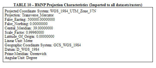
Files downloaded from this site were taken from http://www.maplibrary.org/stacks/ Africa/Ethiopia/index.php and were extracted from their zipped files using WinZip. See Table 10 (below) for imported coordinate system parameters.

Administrative Boundary Areas
-Did not come with the necessary projection files.
-Layer was projected using the following technique:
            ArcToolbox:
                        …Data Management Tools
                                    …Projections and Transformations
                                                …Define Projection
                                                            -Input dataset was selected
                                                            -Coordinate system: Import BMNP
Ethiopia Satellite Image
-Did not come with the necessary projection files.
-Layer was projected using the following technique:
            ArcToolbox:
                        …Data Management Tools
                                    …Projections and Transformations
                                                …Define Projection
                                                            -Input dataset was selected
                                                            - Coordinate system: Import BMNP
Ethiopia Trimmed Satellite Image
-Did not come with the necessary projection files.
-Layer was projected using the following technique:
            ArcToolbox:
                        …Data Management Tools
                                    …Projections and Transformations
                                                …Define Projection
                                                            -Input dataset was selected
                                                            - Coordinate system: Import BMNP

2. Class Data Files

Most of the class data files were already correctly projected in WGS 1984 – UTM Zone 37N. The following rasters/datasets needed to be correctly projected:

Ethiopia DEM
-This DEM needed to have the same projection as the rest of our layers, so the following technique was used:
            ArcToolbox:
                        …Data Management Tools
                                    …Projections and Transformations
                                                …Raster
                                                            …Project Raster
                                                                        -Input raster was selected
                                                                        -Output raster location was defined
                                                                        -Coordinate system: Import BMNP
Africa Country Boundary
-This dataset did not come with the necessary projection files.
-The layer was projected using the following technique:
            ArcToolbox:
                        …Data Management Tools
                                    …Projections and Transformations
                                                …Define Projection
                                                            -Input dataset was selected
                                                            -Coordinate system: Import BMNP
Ethiopia Towns
-The size of this dataset was larger than what we needed.
-We used the Select tool to select Ethiopian towns surrounding BMNP and then exported the selection as its own separate layer.

3. Paul Evangelista’s Files

All of Paul’s files were correctly projected in WGS 1984 – UTM Zone 37N, so no projection modifications were needed. However, a few of the datasets needed additional attribute information. The following describes these processes:

Wolf Packs
First, the number of wolves in each wolf-pack was manually added to our attribute table. This was done by creating a new field titled Num_wolves (Open the Attribute Table for Wolf_packs, select Options, select Add Field, insert field Name, select Type, choose appropriate Field Properties – precision=5 in this case). After creating this field, an edit session was started to input the wolf-pack numbers (Turn on the Editor Toolbar, select the Editor drop-down menu, click on Start Editing, open the Attribute Table for wolf-packs, manually enter the number of wolves in each pack). The number of wolves corresponding with each wolf-pack was taken from the literature, which provided us with a map of wolf-pack counts, as discussed in the literature review section. Secondly, a similar process was completed for wolf-pack vaccination status (i.e. a new field, Vacc_Status, was added to our Wolf_packs layer and updated based on the Wolf_vaccinated_packs layer given to us by Paul Evangelista).

Vegetation Classification Raster
The vegetation raster we received from Paul Evangelista was created and classified by Paul himself along with a few other colleagues. The map was delivered in a zipped file, which was un-zipped via WinZip and then opened and viewed. The vegetation raster was accompanied by an un-projected information layer containing the vegetation classification scheme. Therefore, we had to add the classification scheme to the vegetation raster. In order to do this we followed a similar procedure as stated above with the wolf-pack layer. First we had to add a field by opening the Attribute Table for the vegetation raster. Then we selected Options, selected Add Field, inserted a field Name, selected the Type – text in this case, chose the appropriate Field Properties, and then started an edit session to insert the vegetation classification schemes as denoted by the un-projected classification scheme layer.

Return to top of page