GIS Concepts

Biomapper uses spatially-explicit data in modeling species distribution, which necessitates an understanding of numerous spatial concepts. The data used in this project also involve a number of spatial (and some temporal) concepts related to data (e.g., continuous/discrete, raster/vector), geodesy (datum, coordinate system and projection), topography (elevation, slope and aspect), autocorrelation (spatial and temporal) and error (uncertainty).

Biomapper

Developed in 2002 by Alexandre Hirzel and associates at the University of Lausanne, Switzerland, Biomapper provides a multivariate approach to model the geographic distribution of species based on presence-only data (Hirzel et al. 2002). Biomapper is freely available software. Using environmental variables (e.g., climate, land cover and topography) and GPS locations of species presence, this software utilizes factor analysis to compare locations at which species were detected to the entire study area. Theoretically, Environmental Niche Factor Analysis (ENFA) models conform to the niche concept (Hutchinson 1959), with the niche described as “a hyper volume in multidimensional space of ecological variables within which a species can maintain a viable population”.

Principles and Approach

ENFA does not require data on species absence. Species absence data is often unreliable because species may not be detected even when present, species may be absent even though the habitat is suitable and data with false or pseudo-absences biases models of habitat suitability.

Marginality, Specialization and the Ecological Niche
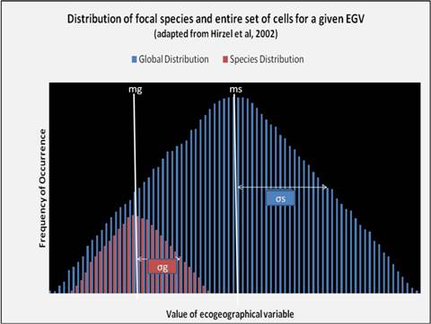
Species presence data points are expected to lie in a subset of the total cells of the study area because species will occupy preferred habitats or areas that lie within their optimal range. By comparing the distribution of values for cells in which a species occurs against the entire set of cells for the same EGV, it is possible to quantify how much these distributions vary with respect to their means and variances.

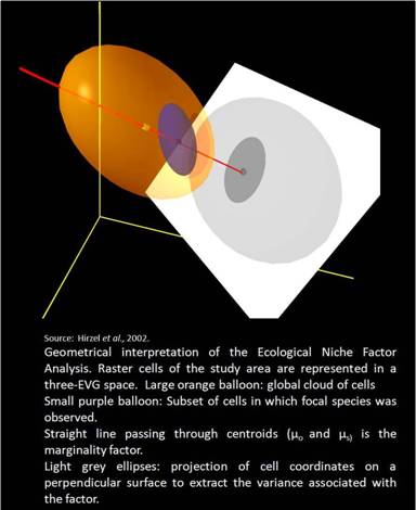
Biomapper allows the quantification of this multivariate niche on any of its axes based on an index of marginality and specialization. Factor analysis has been used to minimize problems associated with multicollinearity and redundancy on account of correlated variables. The use of factor analysis also accounts for interactions between variables (e.g., elevation and temperature) since species may “specialize on a combination of variables, rather than on every variable independently” (Hirzel et al. 2002). The factor analysis procedures used in Biomapper differ slightly from widely used methods such as principal component analysis. The first factor selected in ENFA accounts for all of the marginality of a given species while all subsequent axes maximize specialization.

Marginality: the difference between the species mean and the global mean.

The higher the value of a coefficient, the greater the difference between the species mean and the mean available habitat about a corresponding variable. Values close to 0 indicate that a species prefers values less than the mean with respect to the total area, whereas values close to 1 indicate the contrary. An overall marginality, M’, can be calculated for all EGVs. This allows direct comparisons between marginalities for different species in the same area.

The global tolerance compares the extent to which the habitat of a focal species differs from available conditions based on all EGVs. Low values indicate that species are specialists and can potentially occupy only a fraction of the total area under consideration, whereas high values indicate generalist species.

Specialization: the difference between species variance and global variances (typically the species variance will be smaller).

The first factor extracted in ENFA is the marginality factor. All subsequent factors are specialization factors. A higher absolute specialization value indicates a more restricted range for a species. Each factor has an eigenvalue, λ, associated with it, which is an index for specialization. Eigenvalues decrease with every factor (the highest values being for factor 2). Various criteria are available to facilitate selection, such as a direct comparison with a broken-stick threshold.

The global specialization, s, is the inverse of the global tolerance. It ranges between 1 and infinity and is harder to interpret directly compared to the marginality.

Data Transformation and Normalization
Ecogeographic variables are normalized to the degree possible prior to running analysis in Biomapper. This is because multinormality is an assumption in the extraction of factors using the eigensystem. The box-cox transformation is typically used to transform EGVs in Biomapper so that pixel values for the entire area of interest take on an approximately normal distribution. Although normalization is recommended, Hirzel et al. (2002) note that their method may be robust to deviations from normality.

Computation and Results

Eigenvalues allow one to determine how much variance (between the global and species means) is explained by the factors. Using the score matrix (eigenvectors) provides an indication of how factors are correlated with the variables. Within a factor that explains a large component of the variance, the variables (EGVs) that show the highest coefficient in absolute values in this table provide more information explaining species distribution.

Eigenvalues and eigenvectors are extracted as follows:
1) The W = Rs – 1 * Rg matrix is calculated (Rg – global correlation matrix, Rs – species covariance matrix).
2) From W, the marginality factor is extracted, and the matrix W* is generated. The specialization factors are computed by extracting the eigensystem from W*.

The distribution of eigenvalues is then compared to the distributions from the broken-stick criterion (expected distribution when a stick is broken randomly). Eigenvalues larger than expected for a random distribution are considered to be significant.

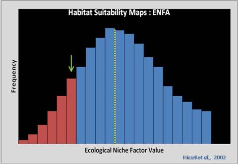
Biomapper allows users to use one of four habitat suitability algorithms, which weigh species distribution data differently. The median algorithm makes the assumptions that optimal habitats are at the median of species distribution on each factor and that these distributions are symmetric.

The default option, median algorithm, is computed by dividing the species range on each factor into 25 classes such that the median separates into exactly two classes. Thereafter, for every point within the environmental space, the observations in the same class or in any other class that is farther apart from the median are counted. These values are then normalized. The final suitability index at each point is calculated using the weighted average of its scores on each dimension (weight – amount of information explained by each dimension).

Habitat suitability map selection criteria
The suitability of a given cell is calculated based on its location (see arrow) compared to the species distribution (histogram) on all selected niche factors. It is calculated as:

Cross-validation of models and habitat suitability maps
The predictive power of habitat suitability maps can be determined using a cross-validation process, which calculates a confidence interval around the predictive accuracy of the habitat suitability models. This is achieved by randomly partitioning species locations into k mutually exclusive sets and then using k-1 (geographically non-overlapping) partitions to compute a new habitat suitability model and the “balance” location data to validate the model. This process is repeated iteratively k times, with different species locations being included in the model and validation datasets each time to generate a number of habitat suitability maps. A comparision of these maps is then used to derive the predictive power of the habitat suitability maps. These processes are carried out based on a method developed by Boyce et al. (2002) and modified by Hirzel et al. (2006).

Components of Biomapper

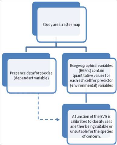
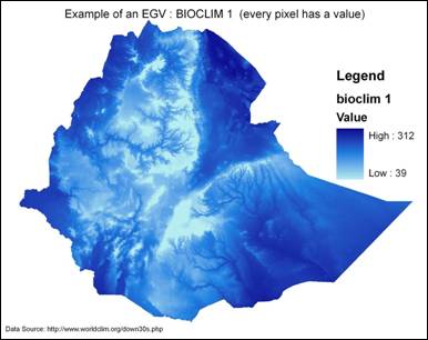
The ecogeographic variable (EGV) map
These are quantitative raster maps (cannot be Boolean or categorical) for environmental variables included in habitat distribution analysis (examples are elevation, mean annual precipitation, Euclidean distance to rivers or density of human populations). Essentially, every pixel has a value. The marginality factor is computed by means for every EGV layer included, and therefore, having categorical data, such as a land cover map, will yield results that are not meaningful. It is recommended that categorical maps be converted into Boolean maps, which are then converted into distance and frequency maps. It is essential that all EVG maps have the same extent and scale.

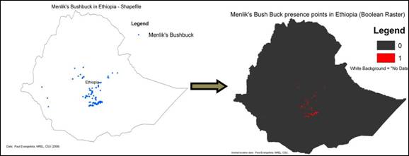
The species map
This is a raster file in Boolean (or binary) code, which contains point locations where the focal species was sighted within the area of interest. A weighted Boolean map may also be used, with integer weighted values for species abundance data. Where reliable absence data is available, it is suggested that more conventional habitat suitability analysis methods, such as generalized linear models, may be used rather than Biomapper.

(return to top of page)

Predictor Variables

BIOCLIM – Bioclimatic variables are derived from monthly temperature and precipitation measurements to create more ecologically meaningful variables. These variables are used in ecological niche modeling (e.g., Biomapper, Maxent). Bioclimatic variables represent annual trends (e.g., annual mean temperature, annual precipitation), seasonality (e.g., annual range in temperature and precipitation) and extreme environmental parameters (e.g., temperature of the coldest and warmest months, precipitation of the wettest and driest quarters). A quarter is a period of three consecutive months.

We used the 19 available bioclimatic variables as predictor layers (e.g., bio1, bio2) in Biomapper.

bio1 – annual mean temperature
bio2 – mean diurnal range (mean of monthly maximum – minimum temperatures)
bio3 – isothermality (bio2 / bio7)
bio4 – temperature seasonality (coefficient of variation)
bio5 – maximum temperature of warmest month
bio6 – minimum temperature of coldest month
bio7 – temperature annual range (bio5 – bio6)
bio8 – mean temperature of wettest quarter
bio9 – mean temperature of driest quarter
bio10 – mean temperature of warmest quarter
bio11 – mean temperature of coldest quarter
bio12 – annual precipitation
bio13 – precipitation of wettest month
bio14 – precipitation of driest month
bio15 – precipitation seasonality (coefficient of variation)
bio16 – precipitation of wettest quarter
bio17 – precipitation of driest quarter
bio18 – precipitation of warmest quarter
bio19 – precipitation of coldest quarter

Source: Hijmans, R.J., S.E. Cameron, and J.L. Parra. 2006. WorldClim version 1.4. University of California, Berkeley, CA. http://www.worldclim.org.

LAND COVER – Land cover classes are derived from the Advanced Very High Resolution Radiometer (AVHRR) satellite imagery. These classes are based on 1) the ratio between surface temperature and NDVI, 2) seasonal metrics derived from the NDVI temporal profile such as length of growing season, 3) a rule-based approach that determines cover type through a series of hierarchical trees based on surface temperature and NDVI values, and 4) annual mean, maximum, minimum, and amplitude values for all optical and thermal channels in the AVHRR data.

There were 11 land cover classes available for Ethiopia, which we reclassified for each species to use as a predictor layer (e.g., “lc_nyala”, “lc_eland”) in Biomapper.

0 – water
2 – evergreen broadleaf forest
4 – deciduous broadleaf forest
6 – woodland
7 – wooded grassland
8 – closed shrubland
9 – open shrubland
10 – grassland
11 – cropland
12 – bare ground
13 – urban and built

Source: Global Land Cover Facility. 1998. Land Cover Classification version 1.0. University of Maryland, College Park, MD. http://glcf.umiacs.umd.edu/data/landcover.

(return to top of page)

Data

Geographic information systems, let alone science, would not be possible without data, and these data are ever more being remotely sensed. Data used in geographic information systems have integrated spatial reference and are available in different formats, which may represent different information or can represent the same information differently. Geographic data is represented in two formats, as raster or vector. We used raster data in Biomapper because species distribution models need data layers to overlay exactly, which is not applicable to vector data. However, many data that are initially available as vector data, such as locations of species saved as point features in shapefiles, go through conversion to raster data. Species distribution models use continuous data, such as elevation, or discrete data, such as land cover, which is usable as nominal or ordinal data with different species distribution models.

GEOGRAPHIC DATA – Information describing the location and attributes of things, including their shapes and representation. Geographic data is the composite of spatial data (information about the locations and shapes of geographic features and the relationships between them, usually stored as coordinates and topology) and attribute data (tabular or textual data describing the geographic characteristics of features).

CONTINUOUS DATA – Data such as elevation or temperature that varies without discrete steps.

Our ecogeographic variable data were mostly continuous data, except for land cover and tree cover.

DISCRETE DATA – Data that represents phenomena with distinct boundaries.

Our data on locations of species and on the boundary of Ethiopia were discrete data as were our data on land cover and tree cover.

NOMINAL DATA – Data divided into classes within which all elements are assumed to be equal to each other, and in which no class comes before another in sequence or importance.

ORDINAL DATA – Data classified by comparative value.

Our data on land cover was originally saved as nominal data but we changed it to ordinal data.

VECTOR – A coordinate-based data model that represents geographic features as points, lines, and polygons. Each point feature is represented as a single coordinate pair, while line and polygon features are represented as ordered lists of vertices. Attributes are associated with each vector feature, as opposed to a raster data model, which associates attributes with grid cells.

SHAPEFILE – A vector data storage format for storing the location, shape, and attributes of geographic features.

POINT FEATURE – In ArcGIS software, a digital map feature that represents a place or thing that has neither length nor area at a given scale.

POLYGON FEATURE – In ArcGIS software, a digital map feature that represents a place or thing that has area at a given scale.

We used data on locations of species saved as point features in shapefiles. We also used data on the boundary of Ethiopia saved as a polygon feature in a shapefile.

RASTER – A spatial data model that defines space as an array of equally sized cells arranged in rows and columns, and composed of single or multiple bands. Each cell contains an attribute value and location coordinates.

CONTINUOUS RASTER – A raster in which cell values vary continuously to form a surface. In a continuous raster, the phenomena represented have no clear boundaries. Values exist on a scale relative to each other. It is assumed that the value assigned to each cell is what is found at the center of the cell.

We used elevation, slope, aspect, temperature and precipitation, solar radiation and net primary productivity as continuous raster data.

DISCRETE RASTER – A raster that typically represents phenomena that have clear boundaries with attributes that are descriptions, classes, or categories. It is assumed that the phenomena that each value represents fill the entire area of the cell.

We used land cover and tree cover as discrete raster data.

GRID – An ESRI data format for storing raster data that defines geographic space as an array of equally sized square cells arranged in rows and columns. Each cell stores a numeric value that represents a geographic attribute (such as elevation) for that unit of space. When the grid is drawn as a map, cells are assigned colors according to their numeric values. Each grid cell is referenced by its x,y coordinate location.

We mostly used data layers (e.g., “bio1”, “precip1”) that were already saved in GRID format.

ASCII - Acronym for American Standard Code for Information Interchange. The de facto standard for the format of text files in computers and on the Internet.

We also used several data layers (e.g., “npp”, “landcover”) that were originally saved in ASCII format.

REMOTE SENSING – Collecting and interpreting information about the environment and the surface of the earth from a distance, primarily by sensing radiation that is naturally emitted or reflected by the earth's surface or from the atmosphere, or by sensing signals transmitted from a device and reflected back to it. Examples of remote-sensing methods include aerial photography, radar, and satellite imaging.

We used many data layers (e.g., “landcover”, “treecover”) that were created by remote sensing with satellite imagery.

Source: Environmental Systems Research Institute. 2006. GIS Dictionary. Environmental Systems Research Institute Inc., Redlands, CA. http://support.esri.com/index.cfm?fa=knowledgebase.gisDictionary.gateway.

* All definitions (shown in blue) are provided verbatim from the GIS Dictionary on ESRI’s website.

(return to top of page)

Geodesy

Mapping geographic data would not be possible without appropriate spatial reference. Spatial reference would not be possible without coordinate systems, datums and projection.

DATUM – The reference specifications of a measurement system, usually a system of coordinate positions on a surface (a horizontal datum) or heights above or below a surface (a vertical datum).

X,Y COORDINATES – A pair of values that represents the distance from an origin (0,0) along two axes, a horizontal axis (x), and a vertical axis (y). On a map, x,y coordinates are used to represent features at the location they are found on the earth's spherical surface.

Our data layers for each species (e.g., “nyala”, “eland”) included x,y coordinates of locations in Ethiopia that were spatially referenced by the global positioning system.

GEOGRAPHIC COORDINATE SYSTEM – A reference system that uses latitude and longitude to define the locations of points on the surface of a sphere. A geographic coordinate system definition includes a datum, prime meridian, and angular unit.

WGS84 – Acronym for World Geodetic System 1984. The most widely used geocentric datum and geographic coordinate system today.

We used several data layers (e.g., “bio1”, “precip1”) that were originally in geographic coordinate system WGS84.

PROJECTED COORDINATE SYSTEM – A reference system used to locate x, y, and z positions of point, line, and area features in two or three dimensions. A projected coordinate system is defined by a geographic coordinate system, a map projection, any parameters needed by the map projection, and a linear unit of measure.

UTM – Acronym for Universal Transverse Mercator. A projected coordinate system that divides the world into 60 north and south zones, 6 degrees wide.

We used several data layers (e.g., “nyala”, “eland”) that were already in projected coordinate system WGS84UTMZone37N, and we projected all of the other data layers into this coordinate system.

PROJECTION – A method by which the curved surface of the earth is portrayed on a flat surface. This generally requires a systematic mathematical transformation of the earth's graticule of lines of longitude and latitude onto a plane. Every map projection distorts distance, area, shape, direction, or some combination thereof.

* All definitions (shown in blue) are provided verbatim from the GIS Dictionary on ESRI’s website.

(return to top of page)

Topography

Topography is very important to species distribution models because many data are correlated to variation in relief. It is possible that temperature and precipitation, because they are correlated to elevation and aspect, would be better predicted by topographic qualities that are quicker and easier to measure. If this were the case, then species distribution models would be simplified by removing extraneous predictor layers, which might also improve model fit with the data.

TOPOGRAPHY – The study and mapping of land surfaces, including relief (relative positions and elevations) and the position of natural and constructed features.

DEM – Acronym for digital elevation model. The representation of continuous elevation values over a topographic surface by a regular array of z-values, referenced to a common datum.

ELEVATION – The vertical distance of a point or object above or below a reference surface or datum (generally mean sea level).

Elevation was already contained in the DEM layer of Ethiopia.

ASPECT – The compass direction that a topographic slope faces, usually measured in degrees from north. Aspect can be generated from continuous elevation surfaces.

Aspect was derived from a DEM layer of Ethiopia in east-west directions and in north-south directions and used as predictor layers (“eastness” and “northness”) in Biomapper.

SLOPE – The incline, or steepness, of a surface. Slope can be measured in degrees from horizontal (0–90), or percent slope (which is the rise divided by the run, multiplied by 100).

Slope was derived from a DEM layer of Ethiopia and used as a predictor layer (“slope”) in Biomapper.

* All definitions (shown in blue) are provided verbatim from the GIS Dictionary on ESRI’s website.

(return to top of page)

Autocorrelation

Geographic data used in species distribution models are unsurprisingly spatially autocorrelated. However, those data that are measured as time-series, such as climatic variables measured monthly (temperature and precipitation), have temporal autocorrelation.

AUTOCORRELATION – The correlation or similarity of values, generally values that are nearby in a dataset. Temporal data are said to exhibit serial autocorrelation when values measured close together in time are more similar than values measured far apart in time. Spatial data are said to exhibit spatial autocorrelation when values measured nearby in space are more similar than values measured farther away from each other.

There were many possible predictor layers (73) in Biomapper and many were correlated, so correlated data layers needed removing before predictor layers were ready to be used as inputs to Biomapper.

TOBLER’S FIRST LAW OF GEOGRAPHY – A formulation of the concept of spatial autocorrelation by the geographer Waldo Tobler, which states “Everything is related to everything else, but near things are more related than distant things.”

* All definitions (shown in blue) are provided verbatim from the GIS Dictionary on ESRI’s website.

(return to top of page)

Error

If we lived in an ideal world, all data would be error-free, but because we live in the real world, all data have errors. To paraphrase a former political appointee known for tortuous speech: there are data we know that we know what the errors are; there are data we know that we do not know what the errors are; and there are data we do not know that we do not know what the errors are. That is, we may be able to deal with the errors that we know are there, we can at least acknowledge the errors that we know are there but do not know what they are, but we are at a loss to deal with the errors that we have not even thought about. These errors cause uncertainty in our data.

ERROR – In a GIS database, a spatial or attribute value that differs from the true value. Error may also be understood as the totality of wrong or unreliable information in a database. Spatial errors are mainly errors in position (feature coordinates are wrong) and topology (features do not properly connect, intersect, or adjoin). Attribute errors are wrong quantities or descriptions associated with features, or missing or invalid values. Errors enter a GIS database through various processes, including data collection (for instance, flawed instruments); data conversion (for example, map digitizing mistakes); data entry and editing; data integration (for example, mixing data at different scales); spatial data processing (for example, inaccuracies caused by generalization); and data analysis (for example, features assigned to inappropriate categories on the basis of flawed criteria).

UNCERTAINTY – The degree to which the measured value of some quantity is estimated to vary from the true value. Uncertainty can arise from a variety of sources, including limitations on the precision or accuracy of a measuring instrument or system; measurement error; the integration of data that uses different scales or that describe phenomena differently; conflicting representations of the same phenomena; the variable, unquantifiable, or indefinite nature of the phenomena being measured; or the limits of human knowledge.

We used data with varying uncertainty about error. We did not collect our own data; we gathered it from other sources, so we cannot be sure of its quality. We are relative certain about the accuracy of the data on locations of species but uncertain about the precision of those data in describing the species distributions prior to modeling. All of our data layers were at the same scale, but one data layer (“npp”) was at a different resolution, so we resampled it but are uncertain about how error might have been introduced to the species distribution model because of it. Although we ourselves might be sources of error in our species distribution models, we feel relatively certain that we are not, but we feel uncertain about error in the data.

* All definitions (shown in blue) are provided verbatim from the GIS Dictionary on ESRI’s website.

(return to top of page)