Invasive Species Exercises: P-Plot

The P-Plot is a mixture of the Modified Whittaker and Nested Pixel Plots.

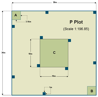
The P-Plot is designed to incorporate nested subplots for monitoring, scattered subplots to represent the entire area being sampled, and square subplots, to mimic the size and shape of one pixel from a satellite image.

the P-Plot is 30 by 30 meters, for a total of 900 square meters in area, with 10 one-square-meter, 2 ten-square-meter, and one 100-square-meter subplots.

• 1 100-meter tape ("Tape 1")
• 2 50-meter tapes ("Tapes 2 and 3")
• 8 Ground stakes
• Meter stick
• 100 square centimeter disc (optional, but useful to represent 1% of the 1 square-meter subplot)
• 10 square-meter subplot frame
• 1 square-meter subplot frame
• Compass
• GPS unit
• Palm Pilot PDA with EcoNab
• Reference materials (dichotomous floristic keys, etc)

1. Identify origin (0,0) (or SE corner) using GPS unit and predetermined UTM coordinate.
2. From the origin (0,0), walk out 100m tape (tape “1”) to 30m at 2700 (or west). This SW corner is point (30,0). When walking out tape, be careful to walk on the left (outside) side of tape to avoid trampling subplots along inside of tape. (Note: it is advisable to walk “wide” left with the tape and at 30 meters line up tape using back-azimuth with previous point to ensure no disturbance of subplots.)
3. From point (30,0), lay out the tape another 30 meters to 60m at 00 (or north). This NW corner point is point (30,30). Take same precautions as above to avoid nested subplots.
4. From point (30,30), lay out tape another 30 meters to 90m at 900 (or east). This NE corner point is point (0,30). Take same precautions as above to avoid nested subplots.
5. From point (0,30), run first 50m tape (tape “2”) 30 meters south (1800) to origin (0,0). This encloses the 900meters squared P-plot. Again, take the same precautions as above to avoid disturbing subplots.
6. From origin (0,0) measure 14.14 meters at 3150 azimuth (NW) to origin of nested C-plot (10,10). To avoid trampling subplots, walk “wide” right of point (10,10). Follow similar procedures as above to properly identify point (10,10).
7. From (10,10), run second 50m tape (tape “3”) 10 meters to point (20,10) on 2700 azimuth. Take care not to stand in a subplot. (Note: there are four 1m2 subplots situated along the outside of nested C-plot. To avoid standing in one while you are setting up C-plot, walk wide right initially, and before 10m, walk wide left. Follow above procedures for identifying point.)
8. From point (20,10) walk tape another 10 meters along 00 azimuth to point (20,20). To avoid disturbing 1m2 subplots, follow procedure noted in step 7.
9. From point (20,20) walk tape another 10 meters along 900 azimuth to point (10,20). To avoid disturbing 1meters squared subplots, follow procedure noted in step 7.
10. From point (10,20) walk tape another 10 meters along 1800 azimuth to point (10,10). To avoid disturbing 1m2 subplots, follow procedure noted in step 7. This encloses the C-plot.
11. Two 10-square-meter plots are set up in the (0,0) (B-plot) and (30,30) (A-plot) corners, respectively. Both plots are 3.16 meters on a side. Thus the outside corners of the B-plot are located at (0,0), 3.16m of tape “1” (aka “1-3.16m”) and 26.84m of tape “2” (2-26.84m). The outside corners of the A-plot are 56.84m of tape “1” (1-56.84m), point (30,30), and 63.16m of tape “1” (1-63.16m). These plots are set up while sampling.
12. The 10 1-square-meter subplots are located at fixed points along each tape. There are six “outside” subplots and four “inside” subplots. The “outside” subplots are located along the inside of the P-plot at locations (tape-distance from tape origin) 1-18m, 1-36m, 1-54m, 1-72m, 1-89m, and 2-18m. The “inside” subplots are located on the outside of the C-plot at 3-0m, 3-10m, 3-20m, and 3-30m. These subplots are setup while sampling.

Sampling Methods:

The ten 1-square-meter subplots are sampled most intensively, with unique biological crusts (optional), plant species, and abiotic cover types identified and recorded.
Biological crusts are identified based on development.
For each crust, percent cover (foliar, basal, or both), average height (cm) of plant species there, and cover type are estimated in the subplot.
For the 10-square-meter and 100-sqaure-meter subplots, presence of all biological crusts, plant species, and abiotic cover types is recorded, but neither cover nor height are estimated on these plots.
The remaining portion of the p-plot is searched for the presence of new cover types and species, with cover and height not estimated.

References:

National Institute of Insvasive Species Science