Invasive Species Exercises: C-Plot

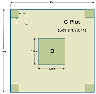
Like the P-Plot, the C-Plot is a hybrid between the Modified Whittaker and Nested Pixel Plots. It incorporates random placement of square subplots within the larger plot, to mimic a pixel of a satellite image, but the C-Plot is scaled down and easier to sample than the P-Plot.
The C-Plot is a 100-square-meter plot, with four 1-square-meter subplots (one in each corner of the plot), and one 10-square-meter subplot in the center of the plot.

Setting up the C-Plot

• Two 50-meter tapes ("tapes 2 and 3")
• Eight ground stakes
• Meter stick
• One 100-square-centimeter disc (optional, but represents 1% of the 1-square-meter subplot)
• One 1-square-meter subplot frame
• Compass
• GPS unit
• Palm Pilot PDA with EcoNab
• Reference materials like floristic keys, etc.

1. Identify origin (0,0) (or SE corner) using GPS unit and predetermined UTM coordinate.
2. From the origin (0,0), walk out 50m tape (tape “1”) to 10m at 270 degrees (or west). This SW corner is point (10,0). When walking out tape, be careful to walk on the left (outside) side of tape to avoid trampling subplots along inside of tape. (Note: it is advisable to walk “wide” left with the tape and at 10 meters line up tape using back-azimuth with previous point to ensure no disturbance of subplots)
3. From point (10,0), lay out the tape another 10 meters to 20m at 0 degrees (or north). This NW corner point is point (10,10). Take the same precautions as above to avoid nested subplots.
4. From point (10,10), lay out tape another 10 meters to 30m at 90 degrees (or east). This NE corner point is point (0,10). Take same precautions as above to avoid nested subplots.
5. From point (0,10), lay out tape another 10 meters to 40m at 180 degrees (or south) back to origin. Take same precautions as above to avoid nested subplots.
6. From origin (0,0) measure 4.84 meters at 315 degree azimuth (NW) to origin of nested D-plot (3.42,3.42).
7. From (3.42,3.42), run second 50m tape (tape “2”) 3.16 meters to point (6.58,3.42) on 270 degree azimuth. (or setup prefabricated 10-square-meter subplot frame)
8. From point (6.58,3.42) walk tape another 3.16 meters along 0 degree azimuth to point (6.58,6.58).
9. From point (6.58,6.58) walk tape another 3.16 meters along 90 degree azimuth to point (10,20). To avoid disturbing 1-square-meter subplots, follow procedure noted in step 7.
10. From point (3.42,6.58) walk tape another 3.16 meters along 180 degree azimuth to point (3.42,3.42), the origin of D-plot. This encloses the D-plot.
11. The four 1-square-meter subplots are located at fixed points along the first tape. The locations of the subplots are 1-0m, 1-9m, 1-19m, and 1-29m. These subplots are setup while sampling.

1. The four 1-square-meter subplots are sampled the most intensely, identifying and recording all unique biological crusts, plant species, and abiotic cover types.
2. Biological crusts are categorized based on development and for each cover type, percent cover (foliar, basal, or both) is estmiated within the subplot.
3. For each plant species within the subplot, average height is estimated.
4. For the 10-square-meter subplot ("D-Plots"), presence of all biological crusts, plant species, and abiotic cover type is recorded, but cover and average height are not observed.
5. The 100-square-meter C-Plot is searched only for the presence of new (to the plot) cover types and species, neither percent cover nor average height is estimated.

The National Institute for Invasive Species Science